Implicit maximum likelihood estimation (IMLE)

An overview of the objective, algorithm, likelihood connection, and synthetic examples for Gaussian, Gaussian-mixture, Cauchy, and misspecified models.

2026-07-11 · interactive figures · companion notebook

IMLE trains implicit generative models without requiring a tractable likelihood. It draws samples from the current model, assigns each data point to its nearest sample, and updates the model to reduce those distances.

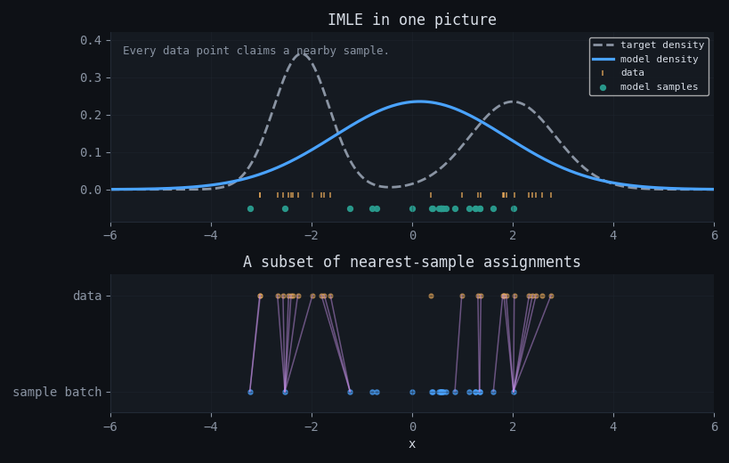
Because matching runs from data points to model samples, every training example must be covered by at least one generated point. This discourages the generator from concentrating probability mass on only a few modes. The examples below show the assignment geometry and the main failure cases.

Contents

1. Why implicit models are hard 2. Core idea and formulas 3. Algorithm and pseudocode 4. Likelihood intuition 5. Animated synthetic cases 6. Interactive examples 7. Failure modes and caveats 8. Summary

1.Why implicit models are hard

The paper studies models of the form $x = T_\theta(z)$ with latent variable $z\sim \mathcal N(0,I)$. This representation supports direct sampling and flexible model classes, but it usually does not provide a closed-form density $p_\theta(x)$ for likelihood optimization.

Training problem: fit a sampler with a likelihood-related objective without evaluating the likelihood itself.

2.Core idea and formulas

Given data $x_1,\dots,x_n$ and i.i.d. model samples $\tilde x_1^\theta,\dots,\tilde x_m^\theta$, define the squared distance from each data point to its nearest sample:

$$R_i^\theta = \min_{j\in[m]} \lVert \tilde x_j^\theta - x_i \rVert_2^2.$$

IMLE chooses parameters by minimizing the expected total nearest-sample distance:

$$\hat\theta_{\rm IMLE} = \arg\min_\theta\; \mathbb E\left[\sum_{i=1}^n R_i^\theta\right] = \arg\min_\theta\; \mathbb E\left[\sum_{i=1}^n \min_{j\in[m]} \lVert \tilde x_j^\theta - x_i \rVert_2^2\right].$$

Each data point is matched to its nearest model sample.

RandomnessThe objective is estimated from a Monte Carlo batch drawn from the current model.

AsymmetryNearest-neighbor matching runs from data points to model samples, not in the reverse direction.

RequirementsNo discriminator, partition function, or explicit density evaluation is required.

InterpretationAlternate nearest-neighbor assignment with gradient updates that move the selected samples toward the data.

IMLE assignments between data points and sampled model points — One-step geometry. Model samples are drawn first, then each data point is connected to its nearest sample.

3.Algorithm and pseudocode

The algorithm alternates between sampling, nearest-neighbor assignment, and several optimization steps with the assignments held fixed:

Compact pseudocode

input: data {x_i}_i=1^n, implicit sampler x = T_θ(z)
initialize θ
for outer iteration k = 1..K:
    draw m i.i.d. samples \tilde x_1^θ, ..., \tilde x_m^θ
    choose a data batch S
    for each i in S:
        σ(i) ← argmin_j ||x_i - \tilde x_j^θ||²
    for inner iteration l = 1..L:
        choose mini-batch \tilde S ⊆ S
        θ ← θ - η ∇_θ [ (n/|\tilde S|) Σ_{i∈\tilde S} ||x_i - \tilde x_{σ(i)}^θ||² ]
return θ

Optimization properties

IMLE uses a single objective and does not require a learned discriminator. When data and model samples are far apart, nearest-sample distances remain nonzero, so the update can still produce useful gradients.

requirementssampling from the model, backpropagation through samples, nearest-neighbor search

behaviordata-to-sample matching encourages mode coverage

costlarge sample batches and repeated nearest-neighbor search can be expensive

4.Likelihood intuition

Under the conditions stated in the paper, the IMLE estimator has the same optimum as maximum likelihood. In the one-point case, increasing model density near a data point $x$ makes nearby samples more likely and lowers the expected nearest-sample distance.

$$\mathbb E[\tilde R] = \int_0^\infty \Pr(\tilde R > t)\,dt.$$

For a nonnegative random variable, a smaller expected distance indicates that more probability mass lies near the data. The multi-point result requires additional assumptions and a more technical argument.

Likelihood connection: IMLE does not use the log-likelihood gradient. It uses a surrogate objective that shares the maximum-likelihood optimum under the paper’s assumptions.

5.Animated synthetic cases

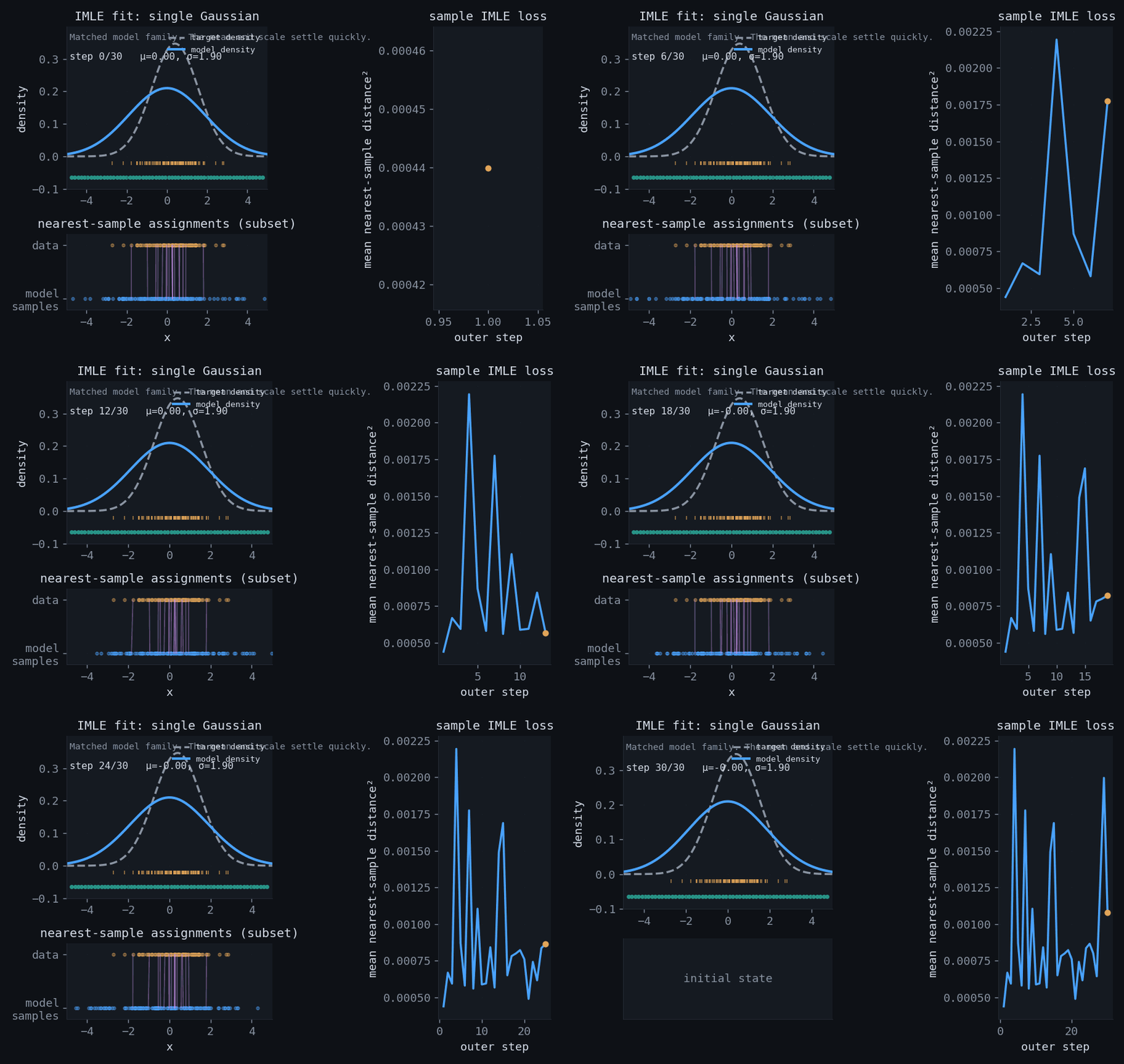
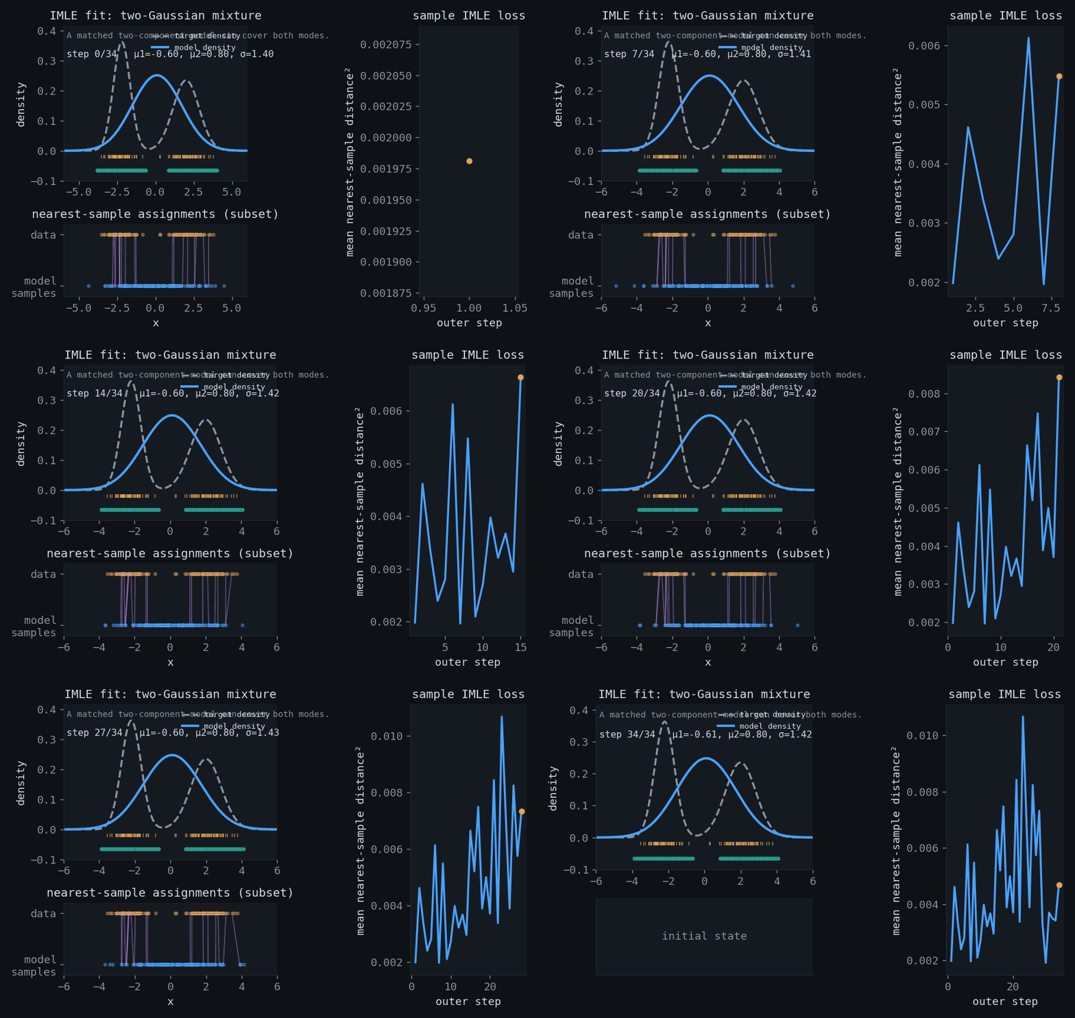
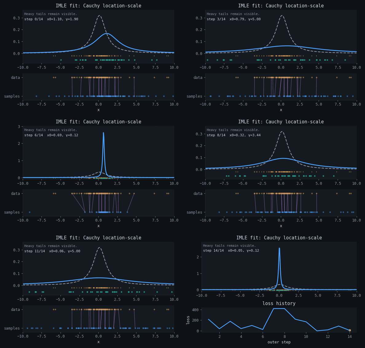
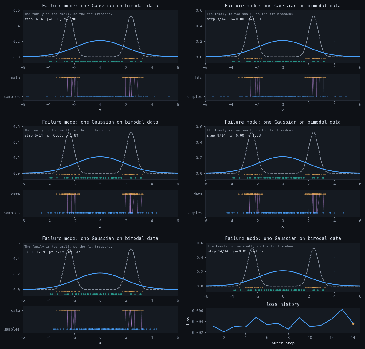
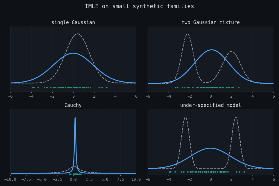
The dashed curve is the target density, the blue curve is the current model density, and the green marks are a fixed set of model samples. The lower strip shows a subset of nearest-sample assignments at each outer step.

Animated fit of a Gaussian with IMLE — **Gaussian.** With a correctly specified model family, IMLE adjusts the mean and scale toward the target.

Animated fit of a Gaussian mixture with IMLE — **Gaussian mixture.** A two-component model can allocate samples to both modes.

Animated fit of a Cauchy distribution with IMLE — **Cauchy.** The objective also applies to a heavy-tailed location-scale family.

Animated failure case fitting a single Gaussian to a bimodal target — **Misspecified model.** A single Gaussian cannot represent two sharp modes, so it broadens and approximates both poorly.

Final IMLE fits on several synthetic targets — Final states from four synthetic experiments. Performance depends on model capacity; a misspecified family can only approximate the target within its representational limits.

6.Interactive examples

The three widgets display nearest-neighbor assignments, current parameter values, and the effect of sample count in low-dimensional examples.

6.1 Assignment geometry

Interactive geometry demo — needs JavaScript.

6.2 Synthetic trainer

Interactive training demo — needs JavaScript.

6.3 Failure lab

Interactive failure demo — needs JavaScript.

7.Failure modes and caveats

Issue	Effect	Implication
Misspecified model	If the family cannot represent the target, IMLE broadens or averages modes within that family.	The model may cover multiple modes while assigning excess probability between them.
Too few sampled points	The Monte Carlo support is sparse, so some data points are matched to distant samples.	The objective estimate becomes noisy even when the model family is correct.
Distance choice	The method optimizes closeness under the chosen metric.	In images, Euclidean distance may not match perceptual similarity.
Nearest-neighbor cost	Large sample sets and repeated searches can dominate runtime.	Approximate nearest-neighbor methods may be needed at scale.

8.Summary

ObjectiveSample from the current model, assign each data point to its nearest sample, and reduce those distances by gradient descent.

Matching directionData points choose model samples, which encourages coverage of the observed modes.

Likelihood connectionUnder explicit assumptions, the IMLE and maximum-likelihood estimators have the same optimum.

LimitationsInsufficient model capacity, small sample batches, and an unsuitable distance metric can all degrade the fit.

Companion material: notebook · synthetic artifacts in artifacts/ · widget source in demo/demo.src.js.